Su Jianlin, a Kimi researcher and the author of rotary position embeddings, has published a short paper titled Notes on the MoE and Attention of K3. It concentrates on the trade-offs Moonshot made in expert architecture, training stability, load balancing and attention design.
K3 carries 2.8 trillion total parameters and 896 routed experts. The model does not call all of them: each token activates 16. The attention stack does not use a single scheme either, alternating KDA layers with gated MLA layers.

Together these choices point at one design principle. Capacity can keep growing, but compute cost must not grow with total parameters and context length at the same rate. More experts mean a finer division of labour. Hybrid attention makes long context affordable.
Scale brings its own problems. As expert counts rise, the router has to pick accurately and stop a handful of experts becoming permanently overloaded. When tokens are dispatched to experts sitting on different GPUs, cross-device traffic climbs fast. Longer context inflates KV cache and attention cost, and low-precision training in BF16 or FP8 saves resources but is more exposed to abnormal activations. So the real question behind K3 is not whether to add experts or swap the attention module, but what control machinery has to be built alongside the expansion.
LatentMoE: paying for a bigger pool
In a conventional mixture of experts, the router selects a few experts per token so the model can hold a very large parameter count while keeping any single computation small. In a real training system, though, those experts live on different GPUs. Once the router has chosen, hidden states must be shipped to the right device. The wider the hidden dimension and the more experts each token activates, the more data moves. At large scale, communication becomes the bottleneck before matrix multiplication does.
LatentMoE changes how a token enters an expert. K3 does not send the full hidden state to routed experts. It compresses first. The main hidden dimension is 7,168, while routed experts compute in a 3,584-dimensional space, with results projected back up afterwards.
The saving is not only in per-expert compute. The weights each expert reads, the activations it handles and the data crossing devices all fall together, and Moonshot spent that budget on a larger pool. A design that would have picked 8 experts from 448 became one that picks 16 from 896. The activation ratio is identical, but the number of combinations is far higher. Several narrow experts can share a token instead of a few wide experts doing every transformation, and specialisation gets finer.
The latent space is also an information bottleneck. Routed experts see a compressed representation, and if the dimension is too narrow some information is lost before the expert sees it. K3 therefore keeps two shared experts that always participate, handling language structure, basic semantics and common reasoning patterns, so hundreds of routed experts do not each relearn the same general computation. LatentMoE is less about making experts smaller than about reorganising the relationship between general capability, specialist capability and communication cost.
Keeping the numbers in range
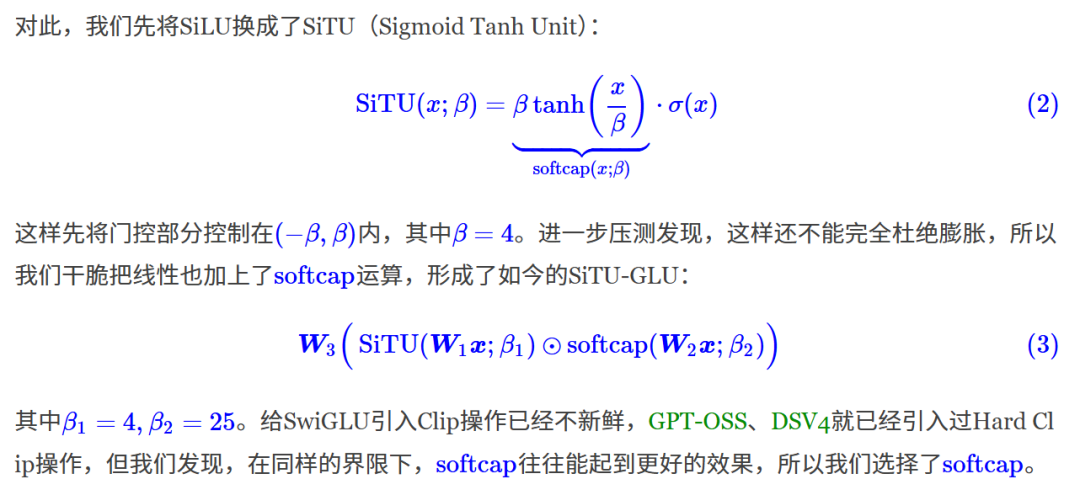
The longer compute path introduced by compression, expert computation, aggregation and re-projection also amplifies numerical wobble in later matrices. K3 adds RMSNorm, SiTU-GLU and Quantile Balancing to turn the design into what Su calls a Stable LatentMoE.
RMSNorm sits after aggregation and before projection back up. Different tokens hit different expert combinations and the router assigns different weights, so aggregate scale can vary considerably. Normalising first gives the routed branch and the trunk a single numerical interface.
Stable overall scale does not rule out local outliers. SwiGLU produces two branches and multiplies them element-wise, so if both are large at the same position the product explodes. That is dangerous in BF16 and FP8 training, where a small number of extreme values consume the dynamic range and squeeze everything normal into a narrow band. SiTU-GLU applies a soft cap: behaviour is preserved while activations are small, and growth slows towards saturation once values enter the danger zone. Unlike a hard clamp, it does not collapse every value above the threshold into the same number.
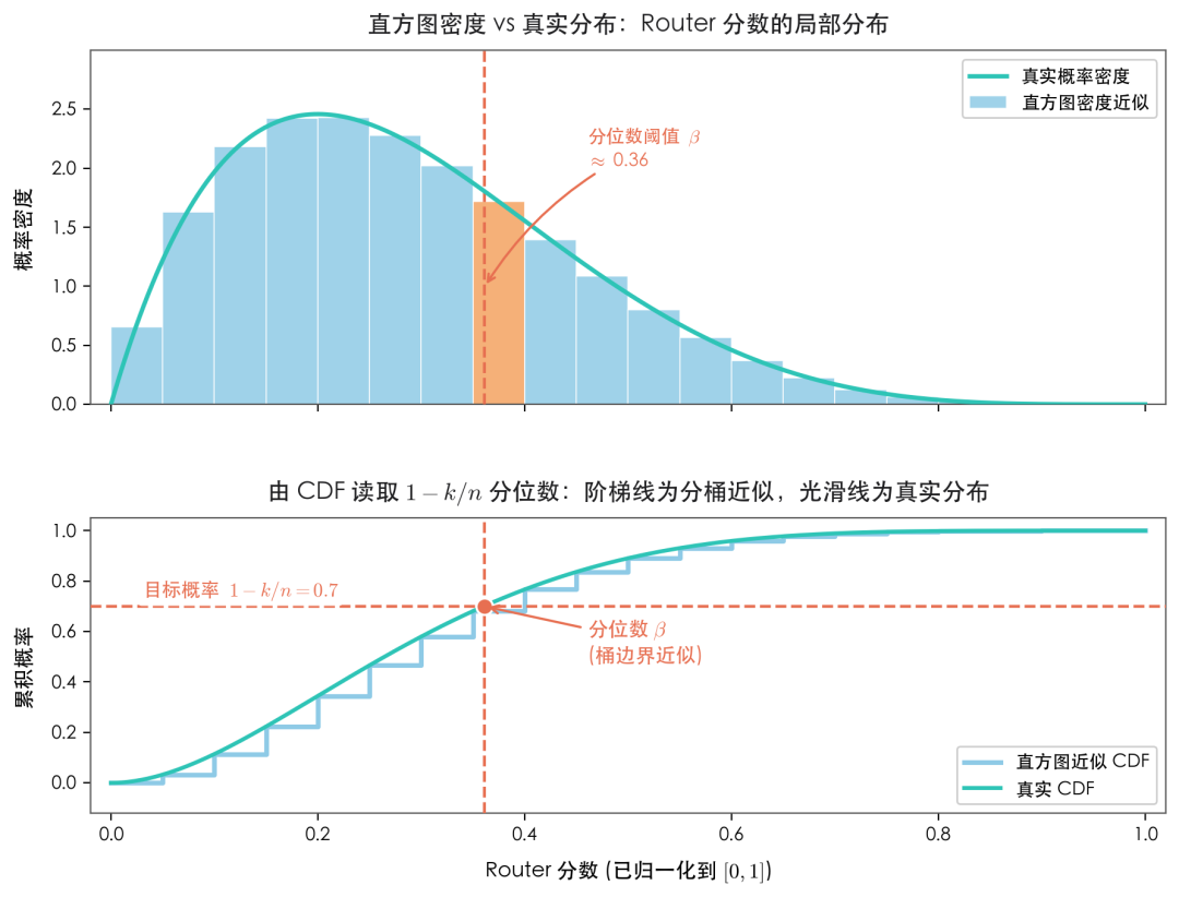
Quantile Balancing handles a different failure. Mixture-of-experts routers create positive feedback. An expert that receives more tokens early gets more gradient, improves, and is then chosen more often. Left alone, a few experts stay overloaded while the rest are undertrained. K2 already used an auxiliary-loss-free balancing method, steering traffic by adjusting selection bias rather than adding a balancing loss that interferes with the router’s semantic learning. But K2’s bias updates behaved like SignSGD, nudging selection probability up or down by a fixed step. With 896 experts, a fixed step cannot be both fast and stable. Quantile Balancing stops probing incrementally and instead reads the distribution of router scores against the top-k threshold, estimating where each expert’s threshold should move to receive its target share. Balancing shifts from empirical feedback to direct distribution solving.
Why K3 can drop RoPE
K3’s attention alternates KDA and gated MLA, roughly one MLA layer for every three KDA layers. They differ in cost, and also in how they hold history. MLA keeps global access to the full record: it compresses the KV cache into a latent space, but the current token can still look up specific content by query. KDA does not store complete representations of every past token, writing history into a fixed-size state maintained through update, forget and overwrite operations. It handles long sequences cheaply, but fixed capacity means some detail is compressed away.
Neither mechanism has to do everything. KDA maintains the continuous state at high frequency, MLA periodically consults the complete history to recover what the fixed state may have dropped.
That division explains why RoPE can be removed from MLA. A pure MLA model needs explicit position modelling between tokens, which is why K2 still relied on RoPE. In K3, KDA updates its state recursively in token order. Older information passes through more propagation, decay and overwriting, while recent information reaches the current position by a shorter path, so order and distance are already partly encoded in the state evolution. MLA no longer has to carry position modelling alone and can spend more capacity on global content matching. Talk of a generalised RoPE does not mean KDA is equivalent to RoPE, only that position information can also be expressed by a sequential state update.
K3 also adds a gate after the MLA output. MLA finds relevant content in history, and the gate decides, based on the current input, which channels are worth writing back to the trunk. The model controls not only what it retrieves but how strongly the retrieval is used.
One curiosity: K3’s NoPE MLA keeps the extra 64-dimension branch originally used for RoPE. In theory it could be deleted. In practice, removing it changes query and key tensor shapes and would ripple through KV cache layout, attention kernels, communication logic and the inference framework. For a 2.8 trillion parameter model with a mature training and deployment pipeline, that is a large revalidation bill. Keeping it is a minimum-change principle: not the most elegant mathematics, but reusable infrastructure and lower risk.
Per-head Muon follows the same spirit. K3 continues to use the Muon optimiser but handles parameters separately per attention head, since heads learn different information patterns and normalising them as one block lets a high-gradient head distort the update scale of the others. The gain may not show up as a headline metric, but the optimiser’s boundaries now match the model’s.
Open questions remain. A low-dimensional latent space can lose information, KDA’s fixed state still forgets detail, and more experts do not automatically produce a matching number of clean capabilities. Efficiency depends on expert communication, low-precision training and specialised kernels, so copying the architecture alone will not reproduce the result. What K3 does show is a clear direction: at trillion-parameter scale with million-token contexts, scaling is no longer about capacity, but about better scheduling of parameters, memory and computation.
Editor’s note: this English report is an adapted translation of a Chinese-language original published by LeiPhone (leiphone.com). Figures, dates and direct quotations follow the source.